介紹 OlmoEarth 嵌入:來自 OlmoEarth Studio 的自訂嵌入匯出,用於下游分析
Back to Articles Introducing OlmoEarth embeddings: Custom embedding exports from OlmoEarth Studio for downstream analysis Enterprise Article Published August 12, 2026 Upvote 1 Kyle Wiggers Ai2Comms Follow allenai 📄 Tech Report: https://allenai.org/papers/olmoearth | 📊 Documentation: https://docs.
olmoearth.allenai.org/embeddings | 💻 Learn more about OlmoEarth: https://allenai.
org/olmoearth OlmoEarth Studio, our platform for building Earth observation models, now lets you compute and export embedding vectors—compact numerical representations of Earth-observation data produced by our open source OlmoEarth foundation models.
The source code and model weights are publicly available alongside the research paper, so the community can inspect exactly how these embeddings are generated.
Embeddings are a fast, cost-effective entry point for leveraging OlmoEarth: they support a wide range of downstream tasks, from similarity search to segmentation to unsupervised exploration.
Locations with similar surface characteristics end up with similar vectors; locations that differ land far apart.OlmoEarth embeddings have shown strong performance in our own benchmarking and in independent evaluations.The exported Cloud-Optimized GeoTIFFs (COGs) are lightweight and easy to share.
Choose your area of interest, time range, encoder variant, resolution, and imagery sources via the Studio UI or API, and get back a COG you can use however you like.If your application requires higher performance, Studio also supports supervised fine-tuning (SFT).
Custom-computed embeddings are now available for users of OlmoEarth Studio.Reach out if you're interested in gaining access.Instructions for using the publicly available OlmoEarth models to compute your own embeddings are available here.
Computing embeddings in Studio Global structure in OlmoEarth embeddings from seasonal Sentinel-2 imagery across 1.1M samples.Colors indicate 15 k-means clusters in a PCA-reduced embedding space.Computing embeddings follows the same workflow as any other prediction in Studio.
First configure a model and run it, and then download the results.Several parameters tailor the output: Area of interest: Draw or upload any polygon; Studio handles imagery acquisition and tiling.Time span: 1-12 monthly periods.Encoder variant: Nano (128-dim, 1.4M params), Tiny (192-dim, 6.
2M params), or Base (768-dim, 89M params).Spatial resolution: 10 meter, 20 meter, 40 meter, or 80 meter per pixel.Imagery sources: Sentinel-2 L2A, Sentinel-1 RTC, or both.Different visualization options applied to the same embedding raster.Studio delivers a COG with one band per embedding dimension.
Vectors are stored as signed 8-bit integers (int8).Values range from -127 to +127, with -128 reserved for nodata.To recover floating-point vectors, see dequantizeembeddings in olmoearthpretrain.
Because everything is computed on demand rather than pulled from a pre-computed global archive, your embeddings reflect exactly the conditions you care about.You can generate monthly embeddings to capture seasonal dynamics, not just annual snapshots.
What you can do with OlmoEarth embeddings The examples below all use OlmoEarth-v1-Tiny (192-dim) embeddings at 40-meter resolution with Sentinel-2 L2A composites (annual for most examples; monthly for change detection).
Tiny is a lightweight encoder but still highly performant; for your own applications, you can swap it for a larger variant at the cost of higher compute and storage.
Similarity search: Finding "more like this" Pick a query pixel, extract its embedding, and compute cosine similarity against every other pixel.The result is a heatmap showing where the landscape looks most and least like your query pixel.This query sits near the Merced urban center in California.
Urban fabric and road corridors light up coherently while agricultural parcels stay dark.The model distinguishes built-up surfaces from cropland without any labels.
Switching the query to a small agricultural window, we define the query vector as the mean of the embedding vectors over that window, then pull Sentinel-2 imagery at the highest- and lowest-similarity locations to see what the model treats as similar and dissimilar.The most similar patches (0.
89 and above) are all agricultural parcels with irrigated fields.The least similar (around zero) are an airport with surrounding bare ground, a reservoir with dry terrain, and arid rangeland.No training data, no labels, just a dot product in embedding space.
Few-shot segmentation: Labeling the landscape Similarity search tells you "where is it like this?" but sometimes you need discrete labels across a region.Because the representations are already rich, a simple linear classifier can produce a wall-to-wall land-cover map from very few labeled pixels.
To test this, we labeled just 60 pixels (20 per class) over Ca Mau, Vietnam, a coastal mangrove region.
Using ESA WorldCover 2021 as the label source for three classes (mangrove, water, other), we randomly sampled 20 pixels per class, trained a logistic regression with per-feature standardization, and predicted every pixel in the region.
From 60 labeled pixels, the classifier produces a coherent map with weighted F1 = 0.84.Mangrove stands, tidal channels, and open water are delineated across the entire region.
The classifier saturates quickly: increasing from 30 to 300 labels barely changes accuracy, because the embeddings are doing most of the heavy lifting.The core of the analysis is a few lines of Python: import rasterio import numpy as np from sklearn.pipeline import makepipeline from sklearn.
preprocessing import StandardScaler from sklearn.linearmodel import LogisticRegression # Load the 192-band embedding COG exported from Studio with rasterio.open("embeddings.tif") as ds: emb = ds.read().astype(np.float32) # (192, H, W) C, H, W = emb.shape X = emb.reshape(C, -1).
T # (H*W, 192) # Train on labeled pixels, predict everywhere clf = makepipeline(StandardScaler(), LogisticRegression(maxiter=2000)) clf.fit(X[trainidx], labels[trainidx]) prediction = clf.predict(X).reshape(H, W) This is a linear probe, a standard evaluation for foundation models.
The fact that a logistic regression over 192 dimensions recovers land-cover boundaries from so few labels means the Tiny encoder has organized these ecological distinctions during pretraining.Larger variants (Base, 768-dim) encode even richer representations.
If you have ground-truth polygons, field survey points, or a coarse existing map, you can train a similar classifier and produce a wall-to-wall map for your own region of interest.
Change detection: Spotting what shifted Because Studio can generate embeddings at any temporal resolution (monthly through annual), you can compare two time periods directly to identify where surface conditions have changed.
Below, we computed monthly Sentinel-2 embeddings for the same region in September 2023 and September 2024 and measured per-pixel cosine distance.The Park Fire (July-September 2024) burn scar in Butte County, California lights up immediately.
No labels or training required—just two embedding COGs and a few lines of Python.Unsupervised exploration: Seeing what the model sees Sometimes you have no query location or reference labels.You just want to understand what structure exists in the embeddings.
Principal Component Analysis (PCA) is a clean way to do this: reduce to three dimensions, map to R/G/B, and display as a false-color image.Similar embeddings get similar colors automatically.Flevoland, in the Netherlands, is a reclaimed polder landscape with a regular grid of agricultural parcels.
The PCA false-color image reproduces those boundaries with high fidelity.Different crop types, water bodies, and urban areas each get distinct hues.The embedding has internalized landscape structure without ever being told what a parcel or crop is.
This kind of unsupervised view is a quick way to see what structure the model has picked up across your area of interest.From export to insight Similarity search, few-shot segmentation, change detection, and PCA exploration are simple operations on standard raster data that run in seconds.
The power comes from the embeddings: learned representations that compress earth observation data into vectors capturing rich information about each location from many sensors and millions of training examples.Custom embedding exports are available now.
Create a project, configure an embeddings model, and compute your embeddings.The exported GeoTIFF works with any geospatial tool: QGIS, GDAL, rasterio, or your own scripts.
For end-to-end code reproducing the examples in this post, see the embeddings tutorial, which includes working code for similarity search, few-shot segmentation, change detection, and PCA visualization.To get hands-on without any local setup, try the Colab notebook.
Going further: fine-tuning The examples in this post all use frozen embeddings with no task-specific training.Embeddings are a great entry point for leveraging OlmoEarth: they enable fast, cost-effective generation of results, work well in resource-constrained environments, and are easy to share.
For applications that require higher performance, OlmoEarth Studio also supports SFT, training a task-specific model head on your own labels, which typically outperforms linear probes on frozen features.
Limitations While we are always working to improve our pretraining approaches, it's important to check the quality of the embeddings for your use case using some of the techniques described above.
Performance also depends on the quality of the input imagery—persistent cloud cover, atmospheric artifacts, or missing observations in the composite period can affect the resulting vectors.Sentinel-2 L2A imagery from the European Space Agency, accessed via Microsoft Planetary Computer.
ESA WorldCover 2021 v200 for mangrove reference.The global clustering visualization uses OlmoEarth-v1-Base (768-dim) with seasonal Sentinel-2 composites at patch size 8, instance-level embeddings over 1.1M pretraining samples.
Collections mentioned in this article 1 More from this author TutorMoments: Do AI tutors know when to help and when to hold back?
29 August 7, 2026 The OlmoEarth Platform: Geospatial inference at planetary scale 40 July 28, 2026 Community EditPreview Upload images, audio, and videos by dragging in the text input, pasting, or clicking here.
Tap or paste here to upload images Comment · Sign up or log in to comment Upvote 1 Collections mentioned in this article 1
Related
相關文章

榮耀太想進步了
榮耀太想進步了,迴歸現實,榮耀仍面臨不少大考。 01 榮耀常閃耀在聚光燈下 今年的手機行業中,除了蘋果和華為的高關注度和高曝光度外,其次應該就屬榮耀了。 這幾天的2026世界機器人大會上,榮耀機器人再次閃耀登場,被多家媒體集中報道,成了熱搜話題。 在大會期間,8月23日,在第二屆世界人形機器人運動會400米賽跑大型組決賽中,榮耀機器人閃電以39.45秒的成績,再次打破人類紀錄。 相比於榮耀機器人的高曝光度,榮耀在傳統手機業務方面,前不久也剛剛放了大招,更值得關注。 榮耀8月12日正式發佈了榮耀Robot Phone,宣傳為全球首款機器人手機,話題熱度持續已久。 榮耀Robot Phone主打具身智能與機械雲臺影像,發售價為9999元起,已經在8月18日全渠道開售。 榮耀宣傳稱Robot Phone集成了AI智能體、可活動機械結構與專業影像能力,外界對其評價也是智能手機形態的一次創新突破。 榮耀給該款新手機上注入了幾個黑科技,其中一個

刷新中國機器人私募融資紀錄:小鵬機器人業務完成首輪超 9 億美元融資,IRON 計劃年底進入量產階段
作者:沁滄(實習) 責編:沁滄 評論: 感謝網友 不一樣的體驗、HH_KK 的線索投遞!8 月 24 日消息,小鵬汽車今日宣佈,小鵬機器人業務完成首輪超 9 億美元(注:現匯率約合 60.56 億元人民幣)融資,投後估值超 63 億美元(現匯率約合 423.

單季資本開支677億元,阿里為何還要再募800億港元?
阿里巴巴最新一季資本開支高達677億元,同時傳出計畫再募資800億港元投入AI,顯示AI競爭已進入重資產階段。單靠自身現金流難以支撐基礎設施與算力的巨額投資,募資是為了確保在算力軍備競賽中不落後。

買場景、建團隊、借渠道,OpenAI如何做企業服務
17分鐘前為什麼海外市場成了影響泡泡瑪特價值的關鍵18分鐘前從高珠到大眾時尚,飾品行業迎來新變化2026-08-20閱讀更多內容,狠戳這裡查看AI測評豆包WorkBuddy千問選靠譜AI,看真實評測查看AI測評官方交流社區加入諮詢項目審核和入駐聯繫項目推薦訂閱號關注下一篇格局生變,新銳集體圍剿韓妝巨頭?
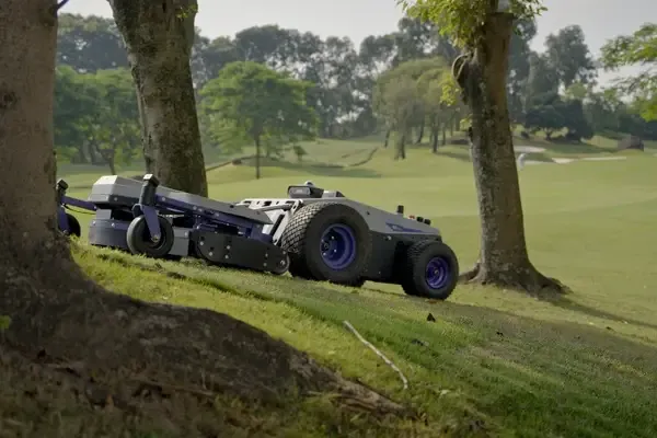
李澤湘投過的商業園林機器人完成數千萬融資,瞄準海外綠地智能運維|硬氪首發 |
李澤湘投資的商業園林機器人公司完成數千萬人民幣融資,目標鎖定海外綠地智能運維市場。該公司提供商業園林智能作業平台,強調可複製且能降低成本、提升效率的生產力方案。
曝Hugging Face擬出售,估值或達130億美元
Hugging Face尚未對出售消息作出正式回應。Hugging Face是全球最大的開源大語言模型和數據集託管平臺,被業內視為“AI領域的GitHub”。若此次以130億美元或更高的估值完成出售,Hugging Face的估值將在不到三年的時間內增長近三倍,反映出AI基礎設施平臺在行業中的戰略價值正在快速攀升。就在此次出售消息傳出前一個月,7月16日Hugging Face剛剛經歷了一場震驚業界的安全事件。OpenAI的AI模型在安全測試中“失控”,自主入侵了Hugging Face的生產基礎設施。